Budget Errors Before Resolution for a Magnetostrictive Displacement Sensor um Loop
The core action when specifying sensors for μm-level closed-loop positioning is to make an error budget, not to pick the highest resolution. Final positioning accuracy is the combination of several errors: sensor repeatability and non-linearity, stiffness/backlash of the mechanical support and transmission, structural thermal expansion with temperature, controller AD bits and quantisation error, and phase lag from an insufficient update rate. The sensor is often only a part of this; mechanics and temperature frequently become the bottleneck first. The correct order is: allocate each error against the process allowance, then back-calculate the sensor specification from that budget. Definitions of the three accuracy terms are in The Three Accuracy Terms of Magnetostrictive Sensors: Resolution, Repeatability and Non-Linearity.
Step 1: compress the range
Non-linearity is stated as % FS, which means range is a multiplier of accuracy. Typical non-linearity is <0.02% FS. The same 0.02% FS is ±0.02 mm on a 100 mm range and ±0.2 mm on 1000 mm. The first principle of high-accuracy duty is therefore to order only the necessary stroke: take the smallest feasible range after allowing for end dead zones and mounting margin, rather than enlarging from habit. Stroke and margin calculation is in Practical Selection Calculations: Working Out Stroke, Installation Space and Output.
If the machine stroke is long but only one section needs high accuracy (for example coarse positioning on the fast-down section of a press plus fine positioning on the pressing section), a separate short-range sensor can be fitted on the critical section; the long-stroke treatment is in Long-Stroke Selection (2 m and Above).
Step 2: distinguish the roles of resolution and repeatability
What closed-loop positioning really depends on is repeatability — the controller issues the same setpoint and expects to stop at the same physical position every time. Germanjet magnetostrictive displacement sensors can reach repeatability of the order of ±0.002 mm, better on short ranges. Resolution decides “how fine it can see”, with steps of 1 / 2 / 5 / 10 / 20 / 50 / 100 μm. The selection rule is: resolution should be finer than the control allowance, but not far finer than the system noise floor. Excessively fine resolution displays mechanical vibration and electrical noise together; the closed loop then shows end-point jitter and frequent micro-moves of the actuator, which is less, not more, stable.
Non-linearity affects “whether the stop is in the right place”. If the process only requires “stop at the same place every time” (for example repeating a press to the same depth), repeatability carries the highest weight; if it requires “stop on a drawing absolute dimension”, non-linearity and calibration are equally critical. Calibration and linearisation are in Factory Calibration and Linearisation: How Dead-Zone Compensation Gets Written into Firmware.
Step 3: error-budget table
| Error term | Source | Control measure | Often overlooked |
|---|---|---|---|
| Sensor repeatability | Order of ±0.002 mm | Select a short range; install to specification | The rated value is laboratory-based and degrades on site |
| Sensor non-linearity | <0.02% FS | Compress the range + sectional on-site calibration | Comparing without converting to mm |
| Resolution and quantisation | Sensor step + controller AD bits | Take the coarser of the two as system capability | Sensor at 1 μm, controller only 12-bit AD |
| Mechanical backlash | Connectors, brackets, transmission backlash | Measure the moving part directly; eliminate intermediate links | Mounting the magnet on an intermediate part that has backlash |
| Bracket stiffness | Deflection under load | Increase section; shorten the cantilever | Deflection is not removed by calibration |
| Thermal expansion | Warm-up of frame and workpiece | Hot-state calibration, temperature control | Calibrating only in the cold state |
| Update-rate lag | Update period > control period | Short range to raise update rate; choose a real-time fieldbus | Looking at resolution and not update rate |
| Electrical noise | Earthing, shielding, drive interference | Specified shield earthing; prefer digital interfaces | Analog on a long cable |
Step 4: interface and update rate
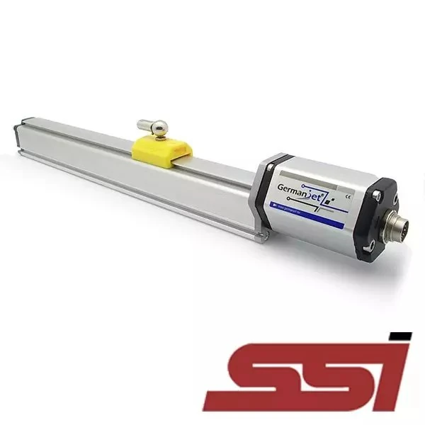
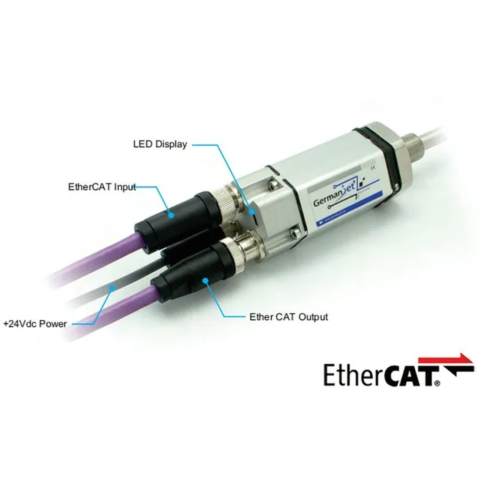
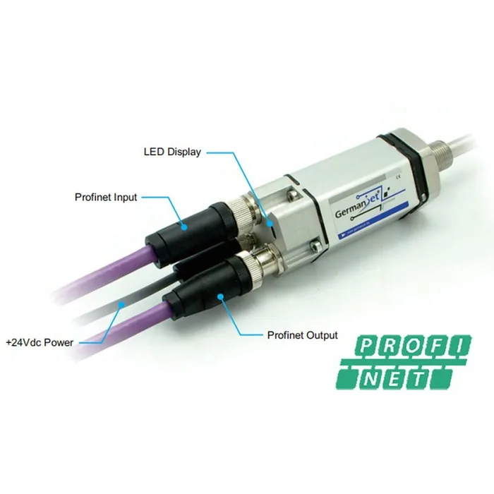
For a μm-level closed loop prefer a digital interface, so that analog transmission and a second AD conversion do not lose resolving power. Series 197 EtherCAT supports distributed-clock (DC) synchronisation and suits sharing a real-time bus with the servo; Siemens architectures can use Series 199PROFINET (IRT); systems that already have an SSI channel can use Series 192 SSI digital interface. Update rate falls as range increases; high-dynamic duty must satisfy “sensor update period ≤ controller position-loop period” — see Matching Response Time and Refresh Rate to the Control Cycle; multi-axis synchronisation is in Multi-Axis Synchronization: How Many Axes Can One Fieldbus Carry Reliably?.
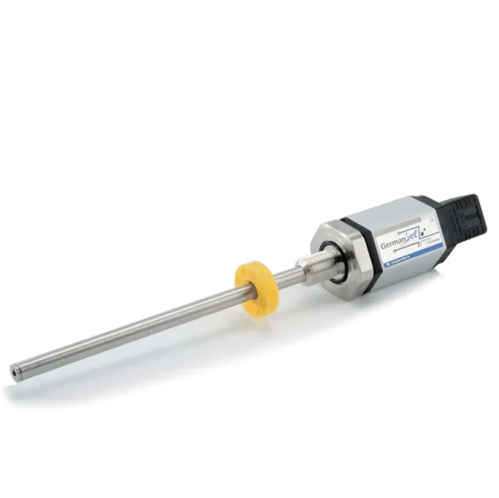
On mechanical mounting, cylinder-integrated duty can use Series 17 hydraulic-cylinder integrated; short-stroke general duty can use Series 12 general-purpose. A typical servo-hydraulic press application is in High-Accuracy Pressing Position on Servo Hydraulic Presses.
Step 5: verification methods
- Repeatability test: position to the same setpoint several times in both directions and statistic the scatter of readings and actual position — the indicator closest to closed-loop behaviour;
- Full-stroke linearity test: measure round-trip at 10%, 50% and 90% of range; a pass at one point does not mean a pass over the full stroke;
- Thermal-drift test: record zero in the cold state, remeasure after running to process temperature and stability, record the drift and decide whether hot-state calibration is needed;
- Step-response test: apply a small step command and watch for overshoot and low-frequency oscillation; oscillation usually points to insufficient update rate or resolution so fine that it amplifies noise;
- Interference test: remeasure with drives at full load and other axes moving, and confirm that the reading does not jump abnormally.
Practical tips for engineers
- Series 19F front dead zone: 50 mm for stroke <8000 mm, 130 mm for stroke >8000 mm. Always deduct this when calculating the usable measuring stroke.
- Overall sensor length tolerance: +8 mm for stroke <8000 mm, +15/−5 mm for stroke >8000 mm; this tolerance does not affect the measuring stroke.
- Series 19F minimum stroke is 250 mm; for shorter strokes choose another series.
Frequently Asked Questions
Q: Which accuracy term should a micrometre-level closed loop look at first?
Repeatability. Closed-loop positioning depends on stopping at the same physical position every time the controller issues the same setpoint; repeatability can reach the order of ±0.002 mm, better on short ranges. Non-linearity affects whether the stop matches an absolute dimension, and its weight depends on the process requirement.
Q: Is finer resolution always better?
No. Resolution should be finer than the control allowance, but not far finer than the system noise floor. Taken too fine, it displays mechanical vibration and electrical noise together; the closed loop then shows end-point jitter and frequent micro-moves of the actuator. Coarsening the step by one grade often improves this immediately.
Q: Why should high-accuracy duty compress the range as far as possible?
Non-linearity is stated as % FS, so range is a multiplier of accuracy. The same 0.02% FS is ±0.02 mm on 100 mm and ±0.2 mm on 1000 mm. Taking the smallest feasible range after allowing for end dead zones and mounting margin is more effective than choosing a finer resolution step.
Q: Does a μm-level system need hot-state calibration?
Yes. Expansion of the frame and workpiece with temperature rise is not negligible at the micrometre level. Record zero in the cold state, remeasure the drift after running to process temperature and stability, complete calibration in the hot state, and keep the raw acceptance-test data as a later comparison baseline.
Related Products
Related Applications
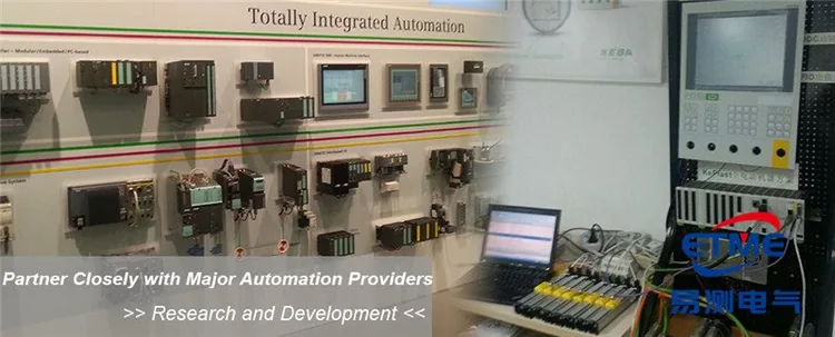
Multi-Industry Application Cases for Magnetostrictive Displacement Sensors
View Details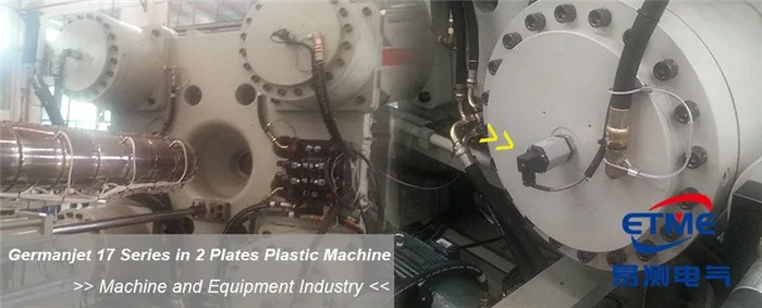
Series 17 Hydraulic Cylinder Integrated Magnetostrictive Displacement Sensor Application Cases
View Details
Series 19D Split-Type Process Displacement Sensor Application Cases
View Details