Magnetostrictive output signals compared: eight interfaces and their trade-offs
Advantages and disadvantages of 4-20 mA, 0-10 V, SSI, Start-Stop, CANopen, Profibus DP, EtherCAT and PROFINET. Look at the controller ports first, then stroke.
Principles, comparisons and application insights for displacement sensors

Advantages and disadvantages of 4-20 mA, 0-10 V, SSI, Start-Stop, CANopen, Profibus DP, EtherCAT and PROFINET. Look at the controller ports first, then stroke.

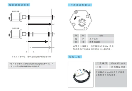
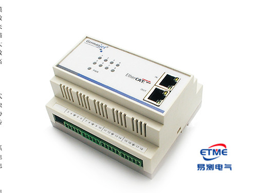
Look at the lamps first: green on / red off is OK; both on means no magnet (including leaving the valid stroke). Then measure voltage or check the magnet — do not strip the head first.

Comparing magnetostrictive and draw-wire displacement sensors on operating principle, accuracy, service life, mounting style and measuring range, with selection advice for cylinder-integrated and external wire applications.

The full Germanjet magnetostrictive range on one page: stroke, accuracy, output signal, protection class and typical applications for the 12 / 13 / 16 / 17 / 18 / 19 series, for fast comparison.

The twin model must be in the same state as the physical asset, and position is the first variable; four data requirements and deployment forms.

Four layers with distinct responsibilities — the field layer produces data, the control layer uses it, the edge layer filters it and the platform layer analyses it — plus the path to the cloud.

Being smart means reporting whether you can be trusted; the four levels of self-diagnostics and where the boundary with functional safety lies.

From waveguide material and high-precision timing circuits to calibration firmware and certification compliance — the real thresholds in magnetostrictive displacement sensors, plus a selection framework that goes beyond the parameter table.

The green benefit is not in sensor power consumption but in the full life-cycle account of less downtime, less scrap and fewer replacements.

SIL assesses the whole safety loop rather than an individual sensor; the relationship between standards and the limits of what redundancy can do.

Networking is not just adding an Ethernet port: the three layers of meaning — value, parameters and status — and the field-level connection path.

Deformation of the position curve for the same motion is a sign of degradation; the observable features and a four-layer judgement method.

Gateways inevitably add latency, failure points and diagnostic gaps; the application boundary and five configuration essentials.

A three-step approach — reflection source, shield grounding, cable routing coupling — with a shield-grounding comparison and a six-symptom checklist.

Three steps to pin down the protocol — check the CPU interface, the communication modules and the existing backbone — with a master-to-product cross-reference table.

Position values are recovered from the physical position of the magnet; parameters rely on non-volatile storage. Includes a comparison of parameter recovery across five protocols.

IO-Link is not a fieldbus but a point-to-point device-level digital link; covers the three data types, IODD and the data storage mechanism.

The controller times the interval between start and stop pulses and converts it; its application boundary and three hard prerequisites.

Reading holding registers and assembling a 32-bit position value, focused on the three most common pitfalls: word order, sign handling and polling period.

Topology configuration is the prerequisite for port-level diagnostics and programming-free device replacement; includes a three-layer diagnostic sequence and common terminating-resistor misconceptions.

Timing details of the master supplying the clock and the sensor shifting data out, including the Gray-to-binary algorithm and bit count configuration.

Explains where the 120 Ω value comes from in terms of transmission line reflection, with a powered-down resistance measurement table and the differing termination requirements of six fieldbuses.

Two main lines — importing the ESI and driving the state machine from INIT to OP — including DC configuration and the IN/OUT chaining order pitfall.

Troubleshooting in three layers — physical layer, address configuration, device diagnostics — including two terminating-resistor traps and a segment isolation method.

The principles of processing-frame pass-through and DC clock compensation, showing which jitter can be eliminated and which is a physical floor.

Node addresses 1–127 must be unique network-wide and the baud rate must be uniform network-wide; includes a configuration procedure and a six-category on-site fault table.

The device name, not the IP address, is the PROFINET identity; includes GSDML configuration, the RT/IRT trade-off and cycle time setting.

The structure of the CANopen object dictionary, the division of labour where position values travel over TPDO and parameters over SDO, and the order in which to bring a device online.

How to allocate multi-magnet position values across TPDOs under the 8-byte frame limit, with mapping steps and synchronous trigger essentials.

A three-step configuration method — import the GSD, set the station address, select the module — including byte order and resolution conversion essentials.

Four boundaries — duty cycle frequency, environmental cleanliness, tolerable downtime and consequence of failure — define where a resistive scale is a legitimate choice.

Long strokes bring four simultaneous constraints — amplified absolute error, reduced update rate, rigidity and transport — and a choice between the flexible and segmented routes.

Build the error budget before picking specifications: compress the range, separate resolution from repeatability, and account for update rate and thermal drift.

Certification is a prerequisite, not paperwork to patch together before delivery — the positioning of four systems and a seven-step verification process.

Three retrofit routes that leave the cylinder intact, six items to measure before starting, signal interfacing options, and four common mechanical installation pitfalls.

Five parameter groups — range, the three accuracy terms, temperature, protection and interface — each with the correct way to read it and the consequences of misreading it.

A four-step calculation method — fix the stroke, the mounting, the environment and the output — plus a pre-order selection checklist you can tick off directly.

Decided by the time budget of three quantities — sensor update period, bus cycle time and controller cycle — with a comparison of synchronization capability by fieldbus.

Pressure selection is based on the system pressure peak, not on the steady-state working pressure. Align by series: Series 16 is 530 bar peak, Series 17 is 600 bar, Series 19 in-cylinder is 600 bar.

The zone classification determines which protection types are permitted, and three further items must be checked: equipment protection level, gas group and temperature class.

The rod is limited by oil temperature and the electronics head by ambient temperature; the two boundaries are independent, and exceeding either one causes failure.

Comparing the selection boundary between magnetostrictive sensors and potentiometric resistive scales in terms of sensing mechanism, failure mode, protection capability and TCO composition.
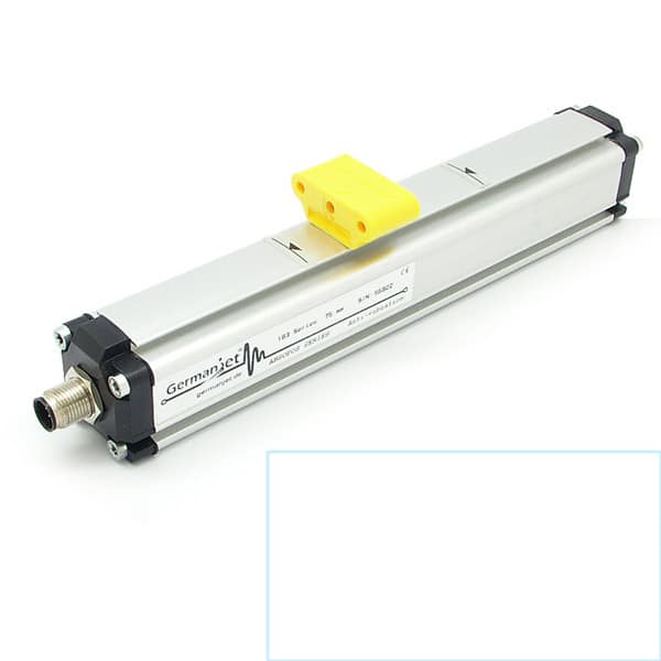
Capacitive and eddy-current sensors measure a millimetre-scale gap; magnetostrictive sensors measure absolute position along a stroke — they are not solutions to the same problem.

Replace a simple price comparison with three dimensions: like-for-like specification comparison, certainty of lead time and spare parts, and technical service responsiveness.

Comparing magnetostrictive sensors, rotary encoders and linear scales against two criteria: whether the measuring chain involves mechanical conversion, and whether re-homing is required.

Lasers depend on an optical path and on reflection from the target surface; magnetostrictive sensors measure inside a sealed rod — their environmental sensitivities are entirely different.

Definition of redundant output, the functional-safety (SIL) background, dual-channel implementation and comparison/validation essentials.

Differences between intrinsic safety, flameproof and dust protection, applicable zones, and deployment of the intrinsic-safety magnetostrictive 17EX.

From injection molding and metallurgy to wind power and process equipment — typical industrial monitoring scenarios for magnetostrictive displacement/position sensors, compared with contact-type solutions, plus explosion-protection deployment essentials.

Waveguide material selection, the advantages of iron-nickel alloy, and the engineering trade-offs between magnetostriction coefficient, temperature drift and service life.

The meaning of IP ratings, how water-ingress testing differs by level, IP69K for high-pressure washdown, and connector protection.
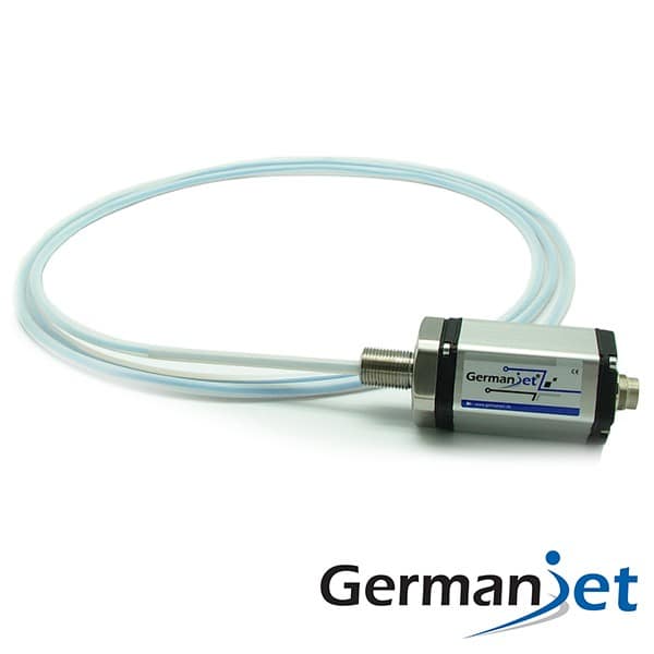
Why EMC is special for magnetostrictive sensors, how strong magnetic fields interfere, shielding and grounding countermeasures, and certification.

The role of factory calibration, how linearisation corrects non-linearity, dead-zone compensation, and why the on-site zero position still has to be set.
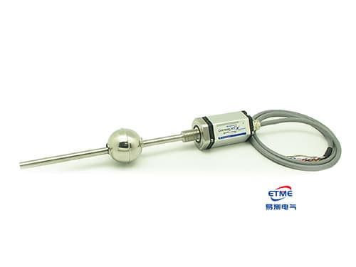
The four modules in the electronics head, how they map to fault symptoms, and a structured troubleshooting approach.

Magnet remanence, temperature coefficient, coaxial gap and anti-loosening essentials, plus high-temperature failure risks.

The difference between operating and storage temperature, the heat tolerance of the electronics head versus the rod, and common selection mistakes.

Multi-magnet measuring principle, Series 19 analogue dual-magnet minimum 76 mm, where it works and where it does not (not usable on multi-stage cylinders), plus fieldbus mapping configuration.

Definitions of response time and refresh rate, how to match them to the control cycle, and the refresh behaviour of fieldbus types.

From node address, PDO/SDO and baud rate to multi-magnet reading — the practical essentials of connecting magnetostrictive displacement sensors to CANopen / EtherCAT, plus on-site pitfalls to avoid.

Magnetostrictive sensors heat themselves after power-up and reach thermal equilibrium in about 30 minutes; this explains the real magnitude of warm-up drift and steady-state temperature effects, and when temperature compensation is genuinely needed.

Where the measuring dead zone comes from, figures for Series 16 / 17 / 19F, and how to keep clear of dead zones when mounting. Do not estimate about 30 mm at each end.

The difference between absolute and incremental position, why magnetostrictive absolute output needs no re-homing after power loss, and what that means in practice.

Clarifies the difference between resolution, repeatability and non-linearity in magnetostrictive displacement sensors and what each means for selection, with on-site pitfalls.

From magnet coaxiality and zero-point calibration to signal cable shielding and grounding — the key steps in installing and commissioning magnetostrictive displacement sensors, plus what to watch when mounting inside hydraulic cylinders.

Organised by symptom, cause and remedy — on-site troubleshooting for no output, fluctuating values, measurement deviation and fieldbus data loss in magnetostrictive displacement sensors.

An objective comparison of magnetostrictive, LVDT and potentiometer displacement technologies across accuracy, service life, stroke, environment and cost, with selection recommendations.

Explains how magnetostrictive displacement sensors measure position, distinguishes the magnetostrictive effect from the Wiedemann effect, and shows why torsion-wave timing and non-contact operation give such long service life.

Compares analog (4-20 mA / 0-10 V) and fieldbus (CANopen / Profibus / EtherCAT / Profinet) outputs for magnetostrictive displacement sensors — pros and cons, suitable applications and protection considerations.